1 August 2026 19 min read

HPLC chromatogram: explanation and worked examples for students

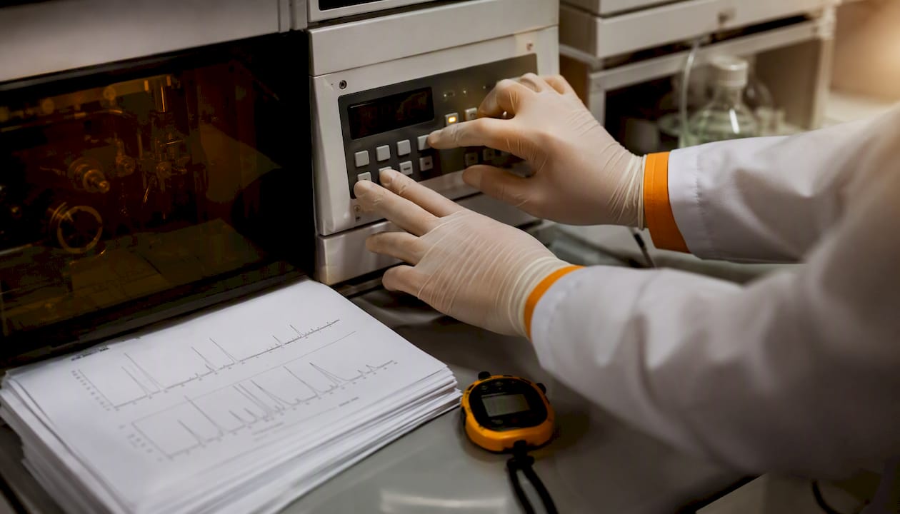
An HPLC chromatogram is a graphical representation of the detector response (y-axis, expressed in mAu with UV detection) plotted against the elution or retention time (x-axis, in minutes). From a single chromatogram you take three kinds of information directly: identification of an analyte via its retention time (tR), quantification via the peak area in combination with a calibration line, and a system check via parameters such as resolution (Rs), theoretical plates (N) and baseline stability. Systems from Waters, Thermo Fisher Scientific and Shimadzu all generate the same type of graph, but the accompanying data software (Empower, Chromeleon and LabSolutions) differs in how peaks are integrated and reported.

The three things you check in the first minute:

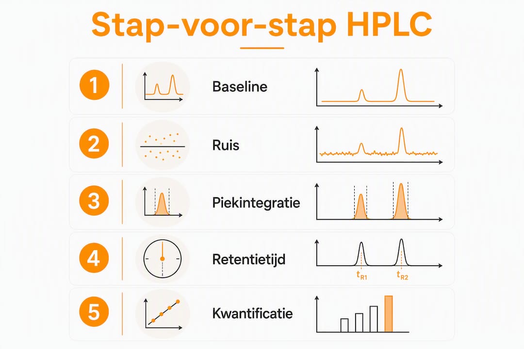
Baseline stability: a flat, low-noise baseline is the precondition for reliable integration.
Retention time against a reference: compare the tR of every peak with that of a reference standard on the same system.
Peak area versus peak height: always use the peak area for quantification, not the peak height.

Pro tip: Check the peak area before the peak height and verify every identification with a certified reference standard. Peak height is more sensitive to variations in peak width caused by column or flow changes; peak area stays more stable.

What does the anatomy of an HPLC chromatogram show?
Which formulas do you use for chromatographic parameters?
How do you go from peak area to concentration?
How does the detector affect the chromatogram?
Isocratic or gradient: what do you see in the chromatogram?
How do you interpret a chromatogram step by step?
Which problems are visible in a chromatogram and how do you solve them?
Two worked examples with complete calculations
What are the core differences between HPLC and GC?
How do you extract retention times and peak areas from a chromatogram?
Step-by-step quantification with a calibration curve
How do you recognise and distinguish overlapping peaks?
Key insights
What students and junior scientists often underestimate
Recommended further reading

What does the anatomy of an HPLC chromatogram show?

The x-axis gives the retention time in minutes, sometimes expressed as elution volume (mL). The y-axis shows the detector response: with UV detection in milli-absorbance units (mAu), with mass spectrometry as ion current, with refractometry as refractive index units. Detector response in mAu is the most widely used unit in routine laboratories.

Core terms you recognise on every plot:

t0 / tM: dead time, the time a non-retained substance needs to pass through the column.
tR: retention time, measured from injection to the peak maximum.
tR’: net retention time, calculated as tR − tM; represents the actual interaction with the stationary phase.
Peak area: the integral under the peak curve; a direct measure of the quantity of analyte.
Peak height: the maximum detector response of a peak; useful for quick comparison but less robust for quantification.
Tailing factor (Tf): a measure of peak shape; ideal is Tf = 1.0, acceptable is 0.8–1.5.

The baseline is the line representing the detector response in the absence of analytes. Noise is the random fluctuation around that baseline. A signal-to-noise ratio (S/N) of at least 3 counts as the limit of detection (LOD); an S/N of 10 as the limit of quantification (LOQ). A drifting baseline, visible as a gradually rising or falling line, indicates thermal instability of the detector, insufficient equilibration of the column, or a changing mobile phase composition.

Software such as Empower (Waters) or Chromeleon (Thermo Fisher Scientific) integrates peaks automatically by drawing a baseline from the start to the end of a peak and calculating the area between them. Visual inspection before final reporting remains necessary: automatic integration sometimes misses a skewed baseline or integrates overlapping peaks as one.

A pair of hands operating the control panel of an HPLC instrument.

Vertical infographic: the main steps of an HPLC chromatogram set out clearly

Which formulas do you use for chromatographic parameters?

The five parameters supporting analytical interpretation and system checking, with their formulas:

Net retention time tR’ = tR − tM

A researcher at a desk, concentrating on calculating chromatographic parameters.

Capacity factor (k) k = tR’ / tM = (tR − tM) / tM

A k value between 1 and 10 is desirable in practice; outside this range the separation is either too fast or too slow.

Selectivity (α) α = k₂ / k₁ (where k₂ > k₁)

α > 1 means two substances are distinguishable; the higher α, the better the selectivity.

Theoretical plates (N) N = 16 × (tR / w)² where w is the peak width at the base or: N = 5.54 × (tR / w₀.₅)² where w₀.₅ is the width at half height

A higher N indicates better column performance. Typical values for a 150 mm C18 column lie between 5,000 and 20,000 theoretical plates.

Resolution (Rs) Rs = 2 × (tR2 − tR1) / (w1 + w2)

Rs ≥ 1.5 is the standard for baseline separation in quantitative methods; Rs = 1.0 gives approximately 4% overlap.

Tailing factor (Tf) Tf = (b / a) where a is the distance from the peak maximum to the leading edge and b the distance to the trailing edge, measured at 5% of the peak height.

Worked example: calculating N and Rs

Suppose two neighbouring peaks with the following values:

Peak 1: tR1 = 5.00 min, w1 = 0.40 min
Peak 2: tR2 = 5.60 min, w2 = 0.44 min
tM = 0.80 min

Step 1 — N for peak 1: N = 16 × (5.00 / 0.40)² = 16 × 156.25 = 2,500 theoretical plates

Step 2 — Rs: Rs = 2 × (5.60 − 5.00) / (0.40 + 0.44) = 2 × 0.60 / 0.84 = 1.43

Rs = 1.43 sits just below the ideal limit of 1.5. For quantification, method optimisation is advisable: increase the column length, lower the flow, or adjust the mobile phase composition.

How do you go from peak area to concentration?

Peak area is a direct measure of the quantity of analyte passing the detector. A factor of 10 difference in peak area corresponds to a factor of 10 difference in concentration, provided the detector response is linear in the working range. Peak height is more sensitive to variations in peak width and therefore less suited to accurate quantification — a common error among students who equate a higher peak directly with a higher concentration.

Step 1: correct integration

Set the baseline limits manually if the software draws a deviating baseline. Filter noise with a suitable time constant, but avoid over-filtering, which artificially widens the peak.

Step 2: calibration line with external standards

Prepare at least four standard solutions with known concentrations. Measure the peak area of each standard under identical conditions.

Standard	Concentration (µg/mL)	Peak area (mAu·s)
S1	—	2,500
S2	1.0	2,490
S3	2.0	4,985
S4	5.00	12,455

Step 3: linear regression and sample calculation

Carry out linear regression: Area = a × Concentration + b. With the data above this gives approximately:

a ≈ 2,490 mAu·s per µg/mL, b ≈ 5 mAu·s (an intercept of virtually zero, which confirms good linearity).

A sample with a measured peak area of 6,200 mAu·s gives:

Concentration = (6,200 − 5) / 2,490 ≈ 2.49 µg/mL

LOD and LOQ are determined conceptually via the signal-to-noise ratio: LOD at S/N = 3, LOQ at S/N = 10. For the validation of quantitative methods, ICH Q2(R1) refers to additional criteria for linearity, accuracy and precision.

Warning: detector response differs per analyte. A UV detector at 254 nm does not respond to substances without an aromatic or conjugated structure. Always use a reference standard of the substance being quantified, or an internal standard with a comparable structure, to determine response factors correctly.

How does the detector affect the chromatogram?

The choice of detector determines which analytes are visible, how sensitive the measurement is, and how the y-axis is interpreted.

UV/Vis detector: measures absorption at a fixed wavelength; reports in mAu. Suitable for aromatic compounds, peptides (214 nm for the peptide band) and most pharmaceutical substances. Simple and robust.
PDA (Photo Diode Array): records a full UV spectrum per time point. Useful for spectral identification and peak purity checking: a peak with an inconsistent spectrum across its shape indicates co-elution.
MS (mass spectrometer, LC-MS): gives mass information per peak, which makes structural confirmation possible. Indispensable for trace analysis and unknown compounds. Ionisation methods such as ESI (electrospray ionisation) or APCI determine which compounds ionise.
RI (refractive index detector): measures the change in refractive index; suitable for non-absorbing analytes such as sugars, polymers and lipids. Sensitive to temperature fluctuations and not usable with gradient elution.

Practical tips per detector:

With UV/Vis, choose the wavelength at the absorption maximum of the analyte for maximum sensitivity; 220 nm gives broad coverage but higher background noise.
Stabilise the RI detector for at least 30–60 minutes before use; even small temperature variations cause baseline drift.
With LC-MS, check the ionisation settings (capillary voltage, temperature) per analyte class; a wrong setting suppresses the signal entirely.

Pro tip: When quantifying, always check that the detector response is linear in the concentration range of interest. An R² value of the calibration line below 0.995 is a signal that the linear range has been exceeded or that the measurement is being disturbed.

Isocratic or gradient: what do you see in the chromatogram?

In isocratic elution the composition of the mobile phase stays constant throughout the run. Retention times are reproducible and the method is easy to validate. Peaks of early-eluting components are narrow and sharp; later-eluting components broaden through longitudinal diffusion.

In gradient elution the ratio of the mobile phase components (water/acetonitrile, for example) changes gradually during the run. Later-eluting peaks are compressed: they elute more sharply than under isocratic conditions, which increases sensitivity. Gradient elution is indispensable for samples with components across a broad polarity range, such as biological extracts or peptide mixtures.

Visible differences in the chromatogram:

Isocratic: even baseline stability, increasing peak width at longer retention times, stable background absorption.
Gradient: a rising or falling baseline through the changing UV absorption of the mobile phase (solvent absorption), compressed peaks for late-eluting components, and a re-equilibration phase at the end of the run.

Choose isocratic for simple samples with components of comparable polarity and where method validation demands simplicity. Choose gradient when the retention times of the components lie too far apart for a single isocratic condition, or when late peaks become too broad for reliable integration.

How do you interpret a chromatogram step by step?

A structured approach prevents errors in the data from being discovered late. The following checklist serves as a minimum protocol for every analytical run.

Check the baseline and noise: is the baseline flat and stable before the first peak? Noise above 0.5 mAu with UV detection calls for investigation (degassing, filter replacement).
Compare retention times with the reference standard: the tR of each analyte may not deviate by more than ±0.1 min from the reference on the same system under the same conditions.
Assess the peak shape: tailing factor between 0.8 and 1.5; a Tf > 2.0 indicates column degradation or strong adsorption to active sites.
Check the integration settings: are the baseline limits correctly placed? Are overlapping peaks correctly separated or integrated as one?
Calculate Rs for critical pairs: Rs ≥ 1.5 for quantitative methods; Rs < 1.0 requires method adjustment.
Check the internal standard or recovery: the peak area ratio of the internal standard may not deviate by more than ±2% between injections.

System suitability acceptance criteria

Parameter	Typical acceptance limit
Theoretical plates (N)	≥ 2000 (method-specific)
Resolution (Rs)	≥ 1.5 for critical pairs
Tailing factor (Tf)	0.8–1.5
RSD peak area (n=6)	≤ 1.0% for quantitative methods
RSD retention time (n=6)	≤ 0.5%

Where one or more parameters fall outside the acceptance limits, do not repeat the run without first identifying the cause. A repeated run with the same system fault yields no usable data.

Which problems are visible in a chromatogram and how do you solve them?

Artefacts in a chromatogram are diagnostic signals, not coincidence. Every pattern points to a specific cause.

Drifting baseline: causes are insufficient column equilibration, temperature fluctuations or a changing mobile phase composition. Solution: equilibrate the column for at least 10 column volumes, check the column oven temperature, and use freshly prepared mobile phase.
High noise: air bubbles in the detector or mobile phase, a contaminated flow cell, or a faulty lamp. Degas the mobile phase with helium or vacuum, clean the flow cell, replace the deuterium lamp in UV detectors.
Ghost peaks: peaks with no corresponding analyte, caused by impurities in the mobile phase, carry-over from a previous injection, or contamination in the injection system. Flush the system with a strong solvent and check the needle wash procedure.
Co-elution: two analytes elute as one broad or asymmetric peak. Increase Rs by lengthening the column, adjusting the gradient, or choosing a different stationary phase. PDA detection helps detect co-elution via spectral inconsistency across the peak shape.
Split peaks: a peak with two maxima, caused by a column void, poor sample dissolution, or too strong a solvent in the sample. Check the column head, dissolve the sample in the mobile phase, and reduce the injection volume.
Broad peaks: too high a flow rate, too large an injection volume, or column degradation. Lower the flow, reduce the injection volume, or replace the column.

Pro tip: Document every change systematically: date, mobile phase batch, column ID and the number of injections on the column. Recurring artefacts can almost always be traced back to a specific batch or a column that has reached the end of its life.

Two worked examples with complete calculations

Example A: identification via retention time

Given values for a peptide analysis:

tM = 0.80 min (measured with a non-retained marker, uracil for example)
tR of the reference standard (GHK-Cu, for example): 6.40 min
tR of the sample: 6.38 min

Net retention time calculation: tR’ (reference) = 6.40 − 0.80 = 5.60 min tR’ (sample) = 6.38 − 0.80 = 5.58 min

The difference of 0.02 min (1.2 seconds) falls within the acceptance limit of ±0.1 min. The peak in the sample is provisionally identified as the target substance. Definitive confirmation requires a second orthogonal method or MS confirmation.

Example B: quantification via an external standard

Use the calibration data from section 4 (a = 2,490 mAu·s per µg/mL, b = 5 mAu·s).

Standard	Concentration (µg/mL)	Measured area (mAu·s)	Calculated area (mAu·s)
S1	—	2,500	2,500
S2	1.0	2,490	2,490
S3	2.0	4,985	4,985
S4	5.00	12,455	12,455
Sample	unknown	6,200	—

Sample concentration = (6,200 − 5) / 2,490 = 2.49 µg/mL

The linearity (R² ≈ 0.9999) confirms that the method is suitable for quantification in this range. Keep the integration settings, the column identification and the batch numbers of the standards with every report: reproducibility can only be demonstrated if the conditions are fully documented.

Pro tip: Save the integration settings as a method file in the data software (Empower, Chromeleon or LabSolutions). Manual adjustments per run are a source of variability and make comparison between runs unreliable.

What are the core differences between HPLC and GC?

Both techniques produce a chromatogram with retention time on the x-axis and detector response on the y-axis, but their fields of application and requirements differ materially.

Characteristic	HPLC	GC
Physical state of sample	Liquid or dissolved in solvent	Volatile or vaporisable
Thermal stability required	No	Yes (temperature range method-specific)
Typical detectors	UV/Vis, PDA, MS, RI	FID, TCD, MS, ECD
Suitable analytes	Polar, ionic, large molecules (peptides, proteins, sugars)	Small, volatile, thermally stable molecules
Mobile phase	Liquid solvent (water/acetonitrile, water/methanol)	Inert carrier gas (helium, nitrogen)

A practical rule of thumb: choose HPLC for non-volatile, thermally labile or polar compounds such as peptides, amino acids and pharmaceutical active substances. GC is the preferred method for volatile organic compounds, residual solvents and gases.

How do you extract retention times and peak areas from a chromatogram?

Extracting quantitative data from a chromatogram is a skill that demands precision, not merely knowledge of the software.

Determining retention time: zoom in on the peak maximum in the data software. Read the tR value at the exact maximum, not on the flank. With asymmetric peaks the maximum can shift visually; use the value the software calculates on the basis of the second derivative.

Extracting peak area: first check the baseline limits the software has placed. A baseline starting too early or too late leads to an over- or underestimate of the area. With overlapping peaks, choose either a perpendicular separation (a vertical line at the valley) or a tangent method, depending on the degree of overlap and the method specifications.

Practical steps in data software:

Open the chromatogram in integration mode (“Integration Events” in Empower or “Peak Integration” in Shimadzu’s LabSolutions, for example).
Set the minimum peak width and threshold to suppress noise without missing real peaks.
Export the integration table with tR, peak area, peak height and tailing factor to a spreadsheet for further calculation.
Compare the extracted tR values with the reference standard on the same system; a deviation greater than ±0.1 min calls for verification.

Step-by-step quantification with a calibration curve

A complete quantification procedure consists of five steps carried out in a fixed order.

Step 1 — Prepare standard solutions: make at least four concentration levels spanning the expected concentration range of the sample. Use certified reference standards of known purity; for peptides, batch-specific CoAs from the supplier are necessary.

Step 2 — Measure the standards: inject each standard at least twice under identical conditions (column, mobile phase, flow, temperature, injection volume). Calculate the mean peak area per concentration level.

Step 3 — Construct the calibration line: plot concentration (x) against mean peak area (y). Carry out linear regression. Accept the line only if R² ≥ 0.999 for quantitative pharmaceutical methods, or R² ≥ 0.995 as a minimum in line with ICH Q2(R1) principles.

Step 4 — Measure the sample: inject the sample under exactly the same conditions as the standards. Read the peak area.

Step 5 — Calculate the concentration: use the regression equation:

Concentration (µg/mL) = (Measured area − b) / a

where a is the slope and b the intercept of the calibration line.

Check that the calculated concentration falls within the calibrated range. If the value lies outside the range, dilute the sample and repeat the measurement.

How do you recognise and distinguish overlapping peaks?

Overlapping peaks are one of the most common challenges in HPLC analysis. They are recognisable by a broad, asymmetric peak with a shoulder or a valley between two maxima, or by a peak whose spectrum (with PDA detection) is inconsistent across the peak shape.

Methods for distinguishing overlapping peaks:

Improve the chromatographic separation: increase Rs by lengthening the column, reducing the particle size of the stationary phase (from 5 µm to 1.8 µm sub-2-micron particles for UHPLC, for example), optimising the gradient, or choosing a different stationary phase (from C18 to C8 or phenyl, for example).

Deconvolution via data software: advanced integration methods such as EMG fitting (Exponentially Modified Gaussian) model the peak shape mathematically and separate overlapping contributions. Software such as Chromeleon (Thermo Fisher Scientific) and Empower (Waters) offers deconvolution options. The method works best when the peaks are partly separated (Rs between 0.5 and 1.0) and the peak shapes are known.

PDA spectral deconvolution: where two overlapping substances have different UV spectra, PDA detection can separate the contributions per wavelength. This is not a full chromatographic separation, but it does give quantitative information per component.

Add an internal standard: an internal standard with a known retention time close to the overlapping peaks helps calibrate the integration limit and correct systematic errors.

With severe overlap (Rs < 0.5), chromatographic method optimisation is the only reliable solution. Deconvolution introduces model-dependent uncertainty that limits the accuracy of quantification.

Key insights

An HPLC chromatogram delivers identification, quantification and a system check in one measurement, provided the baseline is stable, the integration is set correctly, and retention times are compared with certified reference standards.

Point	Details
Identification via retention time	Always compare the tR of the sample with a reference standard on the same system; a deviation ≤ 0.1 min is acceptable.
Quantification via peak area	Use peak area, not peak height, and build a calibration line with at least four standards (R² ≥ 0.999).
Check system suitability	Check N, Rs (≥ 1.5), tailing factor (0.8–1.5) and RSD of peak area (≤ 1.0%) before reporting.
Keep documentation	Save integration settings, column ID, batch numbers and CoAs per run for reproducibility and troubleshooting.
Tackling overlapping peaks	Improve Rs chromatographically or apply EMG deconvolution; at Rs < 0.5, method optimisation is necessary.

What students and junior scientists often underestimate

The technical side of HPLC interpretation can be learnt from textbooks and tutorials. What receives less attention is the discipline of documentation and the value of deliberately varying one parameter at a time.

A common error: repeating a run without understanding the cause of a deviation. If the tailing factor is suddenly 2.3 where it was 1.1 yesterday, repeating is pointless until the cause has been established. Systematic documentation, including column age, mobile phase batch and injection history, makes this kind of diagnosis possible.

Recommended learning materials are the HPLC primers from Waters and the tutorials from Thermo Fisher Scientific, both freely accessible and containing worked example chromatograms. Shimadzu offers practical explanations of integration settings through its LabSolutions documentation. For validation concepts (LOD, LOQ, linearity, precision), ICH Q2(R1) is the primary reference.

Practise with digital integration tools by integrating the same dataset several times with different settings and comparing the outcomes. Compare your own runs with published reference chromatograms of the same compounds. Keep a laboratory notebook recording not only the results, but also the decisions: why was the baseline drawn here, why was this peak integrated as one component?

Pro tip: When optimising a method, always change one parameter at a time. Two simultaneous changes make it impossible to distinguish cause from effect.

Item added to your cart